This 2010 paper have these important results under the realizable case (When the best classifier is perfect):

We see a sharp distinction between the sample complexity required to find a good classifier (logarithmic) and the sample complexity needed to both find a good classifier and verify that it is good. (Section 1 example)

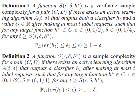
They say definition 2 is a lot easier than definition 1. Definition 1 is equivalent to the case that algorithm return the classifier after some point. Meaning it knows it found a good classifier. In Definition 2 the algorithm suggests classifier at each step that after a certain point is guaranteed to be good. That point however is unknown to the algorithm. We might be able to find an upper bound on the maximum number of labels so that the algorithm found a good classifier using quantities unknown to the algorithm, for example properties of the label distribution.

With Definition 1

Passive learning is known to achieve bound \(O((\frac{d}{\epsilon}) log(\frac{1}{\epsilon}) + (\frac{1}{\epsilon}) log(\frac{1}{\delta}))\).

The hope is to find active learning algorithms that achieve the polylog \(\frac{1}{\epsilon}\) bound. However in many simple cases it has been shown that one need at least \(\frac{1}{\epsilon}\) labels to find a good classifier.

The bound that active learning (CAL) algorithms achieve is as follows:

The label complexity is \(\theta_{h^*}.d.polylog(1/(\epsilon \delta))\), where when run with concept class \(C\) for target function \(h^*\in C\).

With Definition 2

In particular, we show that many common cases have sample complexity that is polylogarithmic in both \(\frac{1}{\epsilon}\) and \(\frac{1}{\delta}\) and linear only in some finite target dependent constant \(\gamma_{h^*}\). This contrasts sharply with the infamous \(\frac{1}{\epsilon}\) lower bounds mentioned above, which have been identified for verifiable sample complexity.

With this definition their goal is to achieve polylog bounds on \(\frac{1}{\epsilon}\) and \(\frac{1}{\delta}\) but potentially linear in \(\gamma_{h^*}\).

With Definition 2 Active learning is always good

With definition 1 we know that we have a lower bound of \(\frac{1}{\epsilon}\), however, they show that with definition 2 have a label complexity of \(o(\frac{1}{\epsilon})\).

Corollary 7. For any \(C\) with finite VC dimension, and any distribution \(D\) over \(X\), there is an active learning algorithm that achieves a sample complexity \(S(\epsilon, \delta, h)\) such that \(S(\epsilon, \delta, h)\) = \(o(\frac{1}{\epsilon})\) for all targets \(h \in C\).

Composing Hypothesis Classes

Assume we have groups of classifiers \(C_1, C_2, \ldots, C_\infty\), and we for each of these groups we have an active learning algorithm that finds a good classifier in \(C_i\) if the optimal classifier is in \(C_i\). The question is how can we merge these algorithms to find a good classifier in \(C\)?

They provide an algorithm that does this. This is the resulting label complexity.

Theorem 8 For any distribution \(D\), let \(C_1, C_2, \ldots\) be a sequence of classes such that for each \(i\), the pair \((C_i, D)\) has sample complexity at most \(S_i(\epsilon, \delta, h)\) for all \(h \in C_i\). Let \(C = \bigcup_{i=1}^\infty C_i\). Then \((C, D)\) has a sample complexity at most

for any \(h\in C\). In particular, Algorithm 1 achieves this, when used with the \(A_i\) algorithms that each achieve the \(S_i(\epsilon, \delta, h)\) sample complexity. This is cool since if we have a algorithm fro each \(A_i\) that is polylog in \(\frac{1}{\epsilon}\) and \(\frac{1}{\delta}\) then their combination would be polylog.

Then they prove a very important and cool theorem. They show that the reverse is also correct. They show that is we have a algorithm that is polylog with definition 2, then we can break the classifier space in a \(C_1, C_2, \ldots\) sequence, that each of \(C_i\) has a polylog algorithm with definition 1 (verifiable active learning).

Theorem 9 For any \((C, D)\) learnable at an exponential rate, there exists a sequence \(C_1, C_2, \ldots\) with \(C = \bigcup_{i=1}^\infty C_i\) , and a sequence of active learning algorithms \(A_1, A_2, \ldots\) such that the algorithm \(A_i\) achieves verifiable sample complexity at most \(\gamma_i polylog_i(\frac{1}{\epsilon\delta})\) for the pair \((C_i, D)\). Thus, the aggregation algorithm (Algorithm 1) achieves exponential rates when used with these algorithms.

Exponential Rates

Some example that Exponential Rates are achievable.

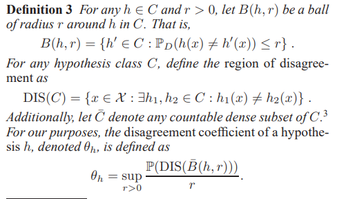
1. Unions of k intervals. for example for k=2 we have classifier that classifies [0.1,0.3] and [0.5,0.7] as + and other points as -. They show that something like this has a disagreement coefficient of \(k+\frac{1}{w(h)}\).
2. Ordinary Binary Classification Trees: Let \(X\) be the cube \([0,1]^n\), \(D\) be the uniform distribution on \(X\), and \(C\) be the class of binary decision trees using a finite number of axis parallel splits.
3. Linear Separators

Composition results

1. They show that if you can achieve a polylog label complexity on some distribution \(D\), you can achieve it in a close distribution \(D'\) such that \(\frac{1}{\lambda}D(A)\leq D'(A) \leq \lambda D(A)\) for some \(\lambda\) and all \(A\).
2. They show that if you can achieve a polylog label complexity on \(D_1\) and \(D_2\), you can achieve polylog label complexity on the linear combinations of them.