Conceptual Themes

They used an example to explain that in active learning we are facing two different scenarios which one of them is very hard for active learning. In the hard scenario the label complexity of active learning is very high and the only thing differentiate between these two scenario is the target function. Therefore, when they report label complexity of algorithms it is usually based on properties of target function.

The example is as follows: Assume our data is 1D data points with binary labels and ew want to learn an interval such that the classifier assigns + to the datapoints inside the interval and - to the datapoints outside of the interval.

They argue that if target function is all -, then it is very hard for us to find the best interval. The only info we have is that the best interval doesn’t include any point we already check its label. So no matter how many samples we use and check their label we are not able to return the best classifier.

Definitions

For any classifier $h$, define $er(h) = P_{XY} ((x, y) : h(x) \neq y)$, called the error rate;
Define $\nu = \inf_{h\in C} er(h)$
Algorithm $A$, achieves label complexity $\Lambda$ if, for every integer $n \geq \Lambda(\epsilon, \delta,P_{XY} )$, if $h$ is the classifier produced by running $A$ with budget $n$, then with probability at least $1 − \delta$, $er(h) \leq \epsilon$.
Define $d = vc(C)$
Define the $\epsilon$-ball centered at $h$ as $B_{C,P}(h, \epsilon) = {g \in C : P(x : g(x) \neq h(x)) \leq \epsilon}$
Define the region of disagreement of $H$ as $DIS(C) = {x \in X : \exists_{h,g \in C} s.t. h(x) \neq g(x)}$
Define the disagreement coefficient of $h$ with respect to $C$ under $P$ as $\theta_h (r_0) = \max(\sup_{r>r_0} \frac{P(DIS(B (h, r)))}{r}, 1)$.
Define $\theta(r_0) = \theta_{f^*}(r_0)$.
Condition 2.3. For some $a \in [1, \infty)$ and $\alpha \in [0, 1]$, for every $h \in C$, $P(x : h(x) \neq f^*(x)) \leq a (er(h) − er(f^*))^{\alpha}$.

Passive Learning

In noisy case we have

Theorem 3.4. The passive learning algorithm ERM(C, .) achieves a label complexity $\Lambda$ such that, for any distribution $P_{XY}$, $\forall \epsilon, \delta \in (0, 1)$,

\[\Lambda(\nu + \epsilon, \delta, P_{XY}) \leq \frac{\epsilon+\nu}{\epsilon^2} \left( d \log \left( \theta(\nu + \epsilon) \right) + \log \left( \frac{1}{\delta} \right) \right)\]

and for the case with $a, \alpha$ we have

\[\Lambda(\nu + \epsilon, \delta, P_{XY}) \leq a \left( \frac{1}{\epsilon} \right)^{2 - \alpha} \left( d \log \left( \theta \left( a \epsilon^{\alpha} \right) \right) + \log \left( \frac{1}{\delta} \right) \right).\]

Lower bounds of passive learning

there exists a distribution $P_{XY}$ for which $er(f^*) = \nu$ and

$\Lambda(\nu + \epsilon, \delta, P_{XY}) \geq \Omega\left(\frac{\nu+\epsilon}{\epsilon^2}(d+\log(1/\delta))\right)$.

Furthermore, for $a ,\alpha$, and sufficiently small $\epsilon, \delta > 0$, there exists a distribution $P_{XY}$ with these values of $a, \alpha$, such that

$\Lambda(\nu + \epsilon, \delta, P_{XY}) \geq \Omega\left(a\left(\frac{1}{\epsilon}\right)^{2-\alpha}(d+\log(1/\delta))\right)$.

Lower bounds of active learning

There exists a universal constant $q \in (0, \infty)$ such that, if $|C| \geq 3$, then for any label complexity $\Lambda$ achieved by an active learning algorithm, for any $\nu \in (0, 1/2)$ and sufficiently small $\epsilon, \delta > 0$, there exists a distribution $P_{XY}$ with $er(f^*) = \nu$ such that

\[\Lambda(\nu + \epsilon, \delta, P_{XY}) \geq q \frac{\nu^2}{\epsilon^2} (d + \log(1/\delta)).\]

Furthermore, for any $a \in [4, \infty), \alpha \in (0, 1]$, and sufficiently small $\epsilon, \delta > 0$, there exists a distribution $P_{XY}$ satisfying Condition 2.3 (in fact, satisfying (2.1) or (2.2), for $\alpha < 1$ or $\alpha = 1$, respectively) with these values of a and $\alpha$, such that

\[\Lambda(\nu + \epsilon, \delta, P_{XY}) \geq q a^2 \left( \frac{1}{\epsilon} \right)^{2 - 2\alpha} (d + \log(1/\delta)).\]

Disagreement-Based Active Learning

where $U$ is defined by

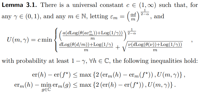
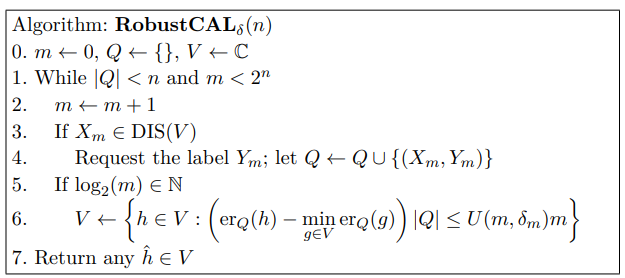
They introduced RobustCAL which is similar to $A^2$ algorithm. It achieves this bound,

$\Lambda(\nu + \epsilon, \delta, P_{XY}) \leq \theta(\nu + \epsilon) \left(\frac{\nu^2}{\epsilon^2} + \log (\frac{1}{\epsilon})\right) \left(d \log (\theta(\nu + \epsilon)) + \log(\frac{\log (\frac{1}{\delta})}{\delta})\right)$.

\[\Lambda(\nu + \epsilon, \delta,P_{XY}) \leq a^2 \theta \left( a \epsilon^{\alpha} \right) \left( \frac{1}{\epsilon} \right)^{2 - 2\alpha} \left( d \log \left( \theta \left( a \epsilon^{\alpha} \right) \right) + \log \left( \frac{\log (a/\epsilon)}{\delta} \right) \right) \log \left( \frac{1}{\epsilon} \right),\]

Note that we have $\theta(r_0) \leq \frac{1}{r_0}$.

The normal analysis of $A^2$ algorithm have $\theta(\nu + \epsilon)^2$ instead of $\theta(\nu + \epsilon)$ but some works shows that a very small changes in $A^2$ can achieve this bound.

Bounding the Disagreement Coefficient

Some properties of Disagreement Coefficient

Let $\epsilon \in (0, \infty)$ and $c \in (1, \infty)$. Then $\theta_h(\epsilon/c) \leq c\theta_h(\epsilon)$ and $\theta_h(\epsilon)/c \leq \theta_h(c\epsilon)$.

They also show that $\theta_h(\epsilon) = O(1)$ is equal to $\theta_h(0) < \infty$,

Second Theorem is about changing distribution a little bit.

Let $\lambda \in (0, 1)$, and suppose $P$ and $P_0$ are distributions over $X$ such that $\lambda P_0 \leq P \leq (1/\lambda)P_0$. For all $\epsilon > 0$, let $\theta_h(\epsilon)$ and $\theta_0^h(\epsilon)$ denote the disagreement coefficients of $h$ with respect to $C$ under $P$ and $P_0$, respectively. Then $\forall \epsilon > 0$,

\[\theta_0^h(\lambda \epsilon) \lambda^2 \leq \theta_h(\epsilon) \leq \frac{\theta_0^h(\epsilon/\lambda)}{\lambda^2}\]

Third Theorem is about merging to distribution.

Suppose there exist $\lambda \in (0, 1)$ and distributions $P^{'}$ and $P^{"}$ over $X$ such that $P = \lambda P^{'} + (1 - \lambda) P^{"}$. For $\epsilon > 0$, let $\theta_h(\epsilon), \theta^{'}_h(\epsilon),$ and $\theta^{"}_h(\epsilon)$ denote the disagreement coefficients of $h$ with respect to $C$ under $P, P^{'},$ and $P^{"}$, respectively. Then $\forall \epsilon > 0$,

\[\theta_h(\epsilon) \leq \theta^{'}_h(\epsilon/\lambda) + \theta^{"}_h(\epsilon/(1 - \lambda))\]

Fourth Theorem is about Merging two classification sets

Let $C^{'}$ and $C^{"}$ be sets of classifiers such that $C = C^{'}\cup C^{"}$, and let $P$ be a distribution over $X$. For all $\epsilon > 0$, let $\theta_h(\epsilon), \theta^{'}_h(\epsilon),$ and $\theta^{"}_h(\epsilon)$ denote the disagreement coefficients of $h$ with respect to $C, C^{'}$, and $C^{"},$ respectively, under $P$. Then $\forall\epsilon > 0$,

\[\max \left\{ \theta^{'}_h(\epsilon), \theta^{"}_h(\epsilon) \right\} \leq \theta_h(\epsilon) \leq \theta^{'}_h(\epsilon) + \theta^{"}_h(\epsilon) + 2\]

The most interesting Lemma is

Lemma 7.12. $\theta_h(\epsilon) = o(1/\epsilon) \iff \Pr \left( \lim_{r \to 0} DIS(B_h(h, r)) \right) = 0.$

Discrete Distribution

every discrete distribution P has $\theta_h(\epsilon) = o(\frac{1}{\epsilon})$.

The proof uses this lemma which is very easy to prove.

Lemma 7.13. $\forall r \in [0, 1], \quad DIS(B(h, r)) \subseteq \left\{x : P(\{x\}) \leq r\right\}$

Theorem 7.14. If $\exists\{x_i\}_{i\in\mathbb{N}}$ in $X$ such that $P(\{x_i : i \in \mathbb{N}\}) = 1$, then $\theta_h(\epsilon) = o(1/\epsilon).$

Asymptotic Behavior

In this section they say lets discuss $P(DIS(B (h, r_0)))$ directly rater than $\theta_h(r_0) = \sup_{r>r_0} \frac{P(DIS(B (h, r)))}{r}$.

They proved these theorems which are easy to understand.

Corollary 7.10. $\theta_h(\epsilon) = O(1)$ if and only if $P(DIS(B(h, \epsilon))) = O(\epsilon)$.

Definition 7.11. For any classifier $h$ and set of classifiers $H$, define the disagreement core of $h$ with respect to $H$ under $P$ as $\partial_{H} h = \lim_{r\to 0} DIS(B_{H}(h, r))$.

Lemma 7.12. $\theta_h(\epsilon) = o(1/\epsilon)$ if and only if $P(\partial_{H} h) = 0$.

Lemma 7.13. For all $r\in [0, 1]$, $DIS(B(h, r)) \subseteq \{x : P(\{x\}) \leq r\}$.

Linear Separators

In this case, we find $\theta_h(\epsilon) = o(1/ \epsilon)$ is guaranteed as long as $P$ has a density; the stronger $\theta_h(\epsilon) = O(1)$ guarantee is obtained as long as the density is bounded, has bounded support, and the separating hyperplane of $h$ passes through the support at a continuity point of the density.

The assumptions seems very reasonable.

Axis-aligned Rectangles

This is like interval learning but in a higher dimension. Assume we have space with $k$ dimensions.

Hanneke found that a certain noise-robust halving-style active learning algorithm achieves a label complexity that, if $p = P(x : f(x) = +1) > 5\nu$, is

\[\frac{k^3}{p}\left(\frac{\nu^2}{\epsilon^2} + 1 \right) \text{polylog} \left(\frac{k}{\epsilon \delta p}\right)\]

Also if $P$ the uniform distribution over $[0, 1]^k$, then

\[\limsup_{\epsilon \to 0} \frac{P(DIS(B(h, \epsilon)))}{\epsilon} < k\]

They also show that

\[\theta_h(\epsilon) \leq \frac{k^3}{p} \cdot \text{polylog} \left(\frac{k}{p \epsilon}\right).\]