Scaling Latent Reasoning via Looped Language Models

The core of the method is a recurrent architecture with a learned mechanism for adaptive computation depth.

LoopLM Architecture

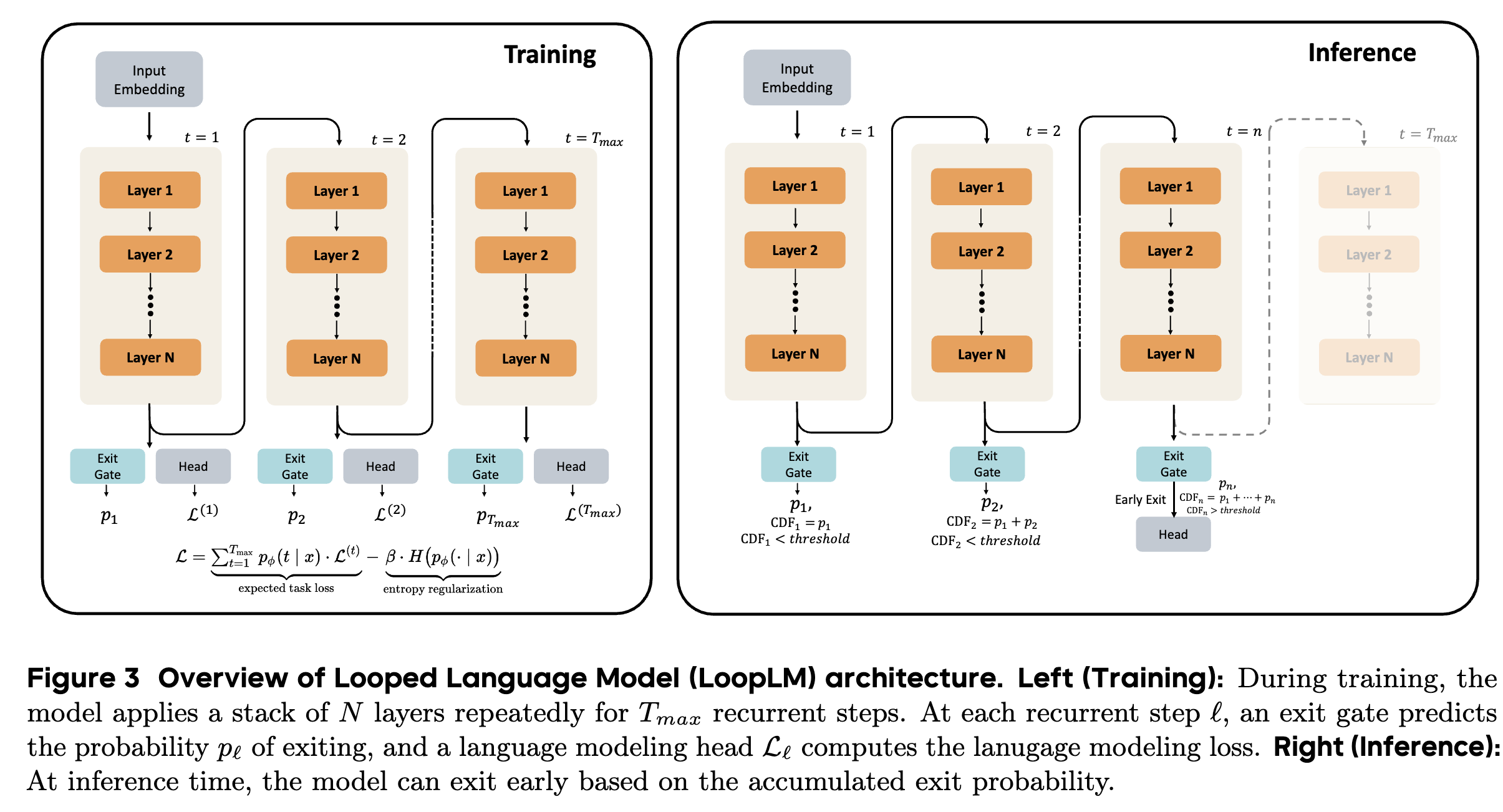
The fundamental idea of LoopLM is to reuse a stack of \(L\) Transformer layers multiple times. A standard non-looped Transformer’s forward pass is \(F(\cdot) := \text{lmhead} \circ M^L \circ \text{emb}(\cdot)\), where \(M^L\) is the composition of \(L\) layers. The LoopLM applies this stack \(t\) times, where \(t\) is the number of recurrent steps or “loops”:

At each recurrent step \(t \in \{1, \dots, T_{\text{max}}\}\), the model produces an output and computes a standard cross-entropy loss for next-token prediction:

where \(h^{(t)}\) is the hidden state after \(t\) loops.

Adaptive Computation via Gating Mechanism

To allow the model to dynamically choose the number of recurrent steps \(t\) for a given input, an “exit gate” is introduced. This gate operates in parallel with the language model head at each step.

1. Instantaneous Exit Probability: At each step \(t\), the gate computes an exit probability \(\lambda_t(x)\) based on the final-layer hidden state \(h^{(t)}\): \(\lambda_t(x) = \sigma(\text{Linear}_\phi(h^{(t)})) \in (0, 1)\) where \(\phi\) are the gate parameters.

2. Exit Distribution: These per-step probabilities are combined to form a valid discrete probability distribution \(p_\phi(t \mid x)\) over the exit steps \(\{1, \dots, T_{\text{max}}\}\). The probability of not exiting in the first \(t\) steps (survival probability) is \(S_t(x) = \prod_{j=1}^t (1 - \lambda_j(x))\). The probability of exiting at step \(t\) is then: \(p_\phi(t \mid x) = \begin{cases} \lambda_t(x) S_{t-1}(x) & \text{if } t < T_{\text{max}} \\ S_{T_{\text{max}}-1}(x) & \text{if } t = T_{\text{max}} \end{cases}\) This ensures that \(\sum_{t=1}^{T_{\text{max}}} p_\phi(t\mid x) = 1\).

3. Inference: During inference, a quantile-based policy is used. Given a threshold \(q \in [0, 1]\), the model exits at the first step \(m\) where the cumulative distribution function \(\text{CDF}(m\lvert x) = \sum_{t=1}^m p_{\phi}(t \rvert x)\) exceeds \(q\).

Two-Stage Training Objective

The model and the gating mechanism are trained in two stages.

Stage I: Entropy-Regularized Objective

During pre-training, the model is trained with an objective that combines the expected task loss across all steps with an entropy regularizer for the exit distribution. The total loss \(\mathcal{L}\) is:

where \(H(p_\phi(\cdot\lvert x)) = - \sum_{t=1}^{T_{\text{max}}} p_\phi(t \rvert x) \log p_\phi(t\mid x)\) is the entropy of the exit distribution. The coefficient \(\beta\) balances the trade-off between task performance and encouraging the model to explore different computation depths.

Stage II: Focused Adaptive Gate Training

After the main pre-training, the LM parameters are frozen, and only the exit gate parameters \(\phi\) are fine-tuned. This stage trains the gate to make termination decisions based on realized performance improvements.

1. Loss Improvement Signal: The improvement in the (detached) per-token loss from step \(t-1\) to \(t\) is calculated: \(I_i^{(t)} = \max(0, \mathcal{L}_{i, \text{stop}}^{(t-1)} - \mathcal{L}_{i, \text{stop}}^{(t)})\)

2. Ideal Continuation Probability: This improvement signal is converted into a soft target label \(w_i^{(t)} \in [0,1]\) indicating whether to continue (\(w_i^{(t)} \approx 1\)) or exit (\(w_i^{(t)} \approx 0\)): \(w_i^{(t)} = \sigma(k \cdot (I_i^{(t)} - \gamma))\) where \(k\) is a slope parameter and \(\gamma\) is a threshold.

3. Adaptive Loss: The gate is trained using a binary cross-entropy loss to match its continuation probability, \(1 - \lambda_i^{(t)}\), to the ideal label \(w_i^{(t)}\): \(\mathcal{L}_{\text{adaptive}}^{(t)} = -\frac{1}{M} \sum_{i=1}^M \left[ w_i^{(t)} \log(1 - \lambda_i^{(t)}) + (1 - w_i^{(t)}) \log(\lambda_i^{(t)}) \right]\)

Training Pipeline and Stability Measures

• Recurrent Step Reduction: Initial experiments with 8 recurrent steps showed instability (loss spikes). The number of steps was reduced to 4 for the main training phases to balance computational depth and stability.
• Stability-Driven Upcycling: To create the 2.6B model from a 24-layer checkpoint, layers were duplicated to 48. The recurrent structure makes this upcycling process smoother than in standard Transformers.
• KL Divergence Coefficient Reduction: The coefficient \(\beta\) was reduced from 0.1 to 0.05 in later stages to decrease conflicting gradients between the task loss and the KL penalty, allowing the model to learn more natural depth patterns.

Efficient Inference with KV Cache Sharing

A naive implementation of LoopLM would require a separate KV cache for each of the \(T_{\text{max}}\) recurrent steps, leading to a \(T_{\text{max}}\)-fold increase in memory usage. The paper investigates KV cache sharing strategies during the auto-regressive decoding phase.

• Finding: While dedicated KV caches are necessary during the prompt processing (prefill) phase, they can be shared during token generation.
• Method: Reusing only the KV cache from the final (4th) recurrent step or an averaged KV cache across all steps results in minimal performance degradation while reducing the memory footprint by 4x, making the models practical for deployment. Using the first-step cache leads to a catastrophic performance collapse.

Here they give it away that during inference they always compute 4 recurents even if the model generates the token in the first recurrence.